Overview Fixed Income Project
Introduction
Thank you for your interest in quantiko-computing.com, a web-based valuation service for
financial instruments offered by Quantiko GmbH for registered users. The following notes will quickly walk you through its
features.
The Fixed Income Project on quantiko-computing.com is about the valuation of interest rate and FX
derivatives like single-currency swaps, cross-currency swaps and FX forwards in a multi-curve
environment, and the market risk associated with those instruments.You can define market data scenarios and see how portfolios fare under
those scenarios including an attribution of profits or losses to single risk factors. You can also easily upload market data, scenarios,
and trades from text files in JSON format. This makes the service a flexible tool - for instance for portfolio risk analysis or for validation tasks.
Conventions
On some of the web pages you might enter data in web forms or upload data from a file. Please stick to the following conventions when you provide data to the service.
- Dates are displayed and supposed to be entered in ISO format YYYY-MM-DD.
- The decimal separator is the point.
- Zero rates/yields are displayed and supposed to be entered as fractions of one, i.e. -0.001 means -0.1% or -10bp (basis points).
- Tenors are displayed and supposed to be entered with small letter, e.g. 5d, 2w, 3m, 10y.
- Names for portfolios, scenarios, instruments etc. must not contain special characters.
- Each currency pair has a standard quote convention, for instance the rate for EURUSD is the number of USD for one EUR. In this example EUR is the base currency while USD is the quote currency . We will also use the terms domestic currency for the quote currency and foreign currency for the base currency. For USDJPY USD is the foreign (base) currency and JPY is the domestic (quote) currency.
Market Data
The service comes without real market data. The screenshots shown here and the example upload file were produced with mock
market data.
For this we took exchange rates and general interest rate levels (mostly government bond yields) published by central banks and applied some
arbitrary constant spreads to arrive at a proxy for a multi-curve set-up for several currencies. Feel free
to upload realistic market data for yourself (for example using the upload tool) — but please kindly consider the section Submitted Data
in the Terms of Use before you upload any data to quantiko-computing.com.
Feedback
We'd love to hear from you. Please do not hesitate to send queries, suggestions or bug reports to computing (at) quantiko.de.Navigation Bar, Reference Date and Home Screen
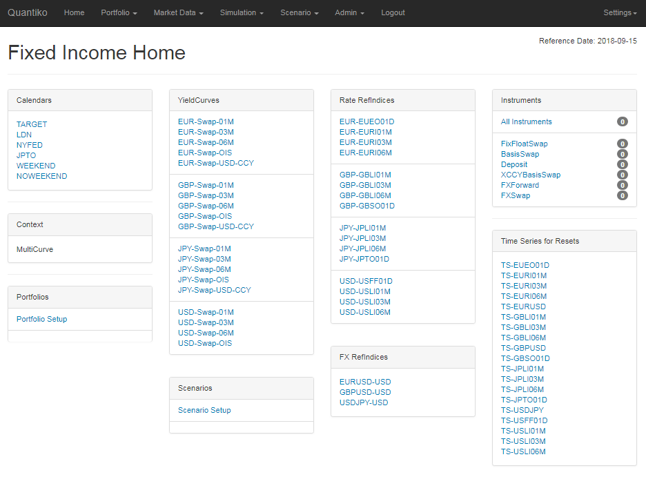
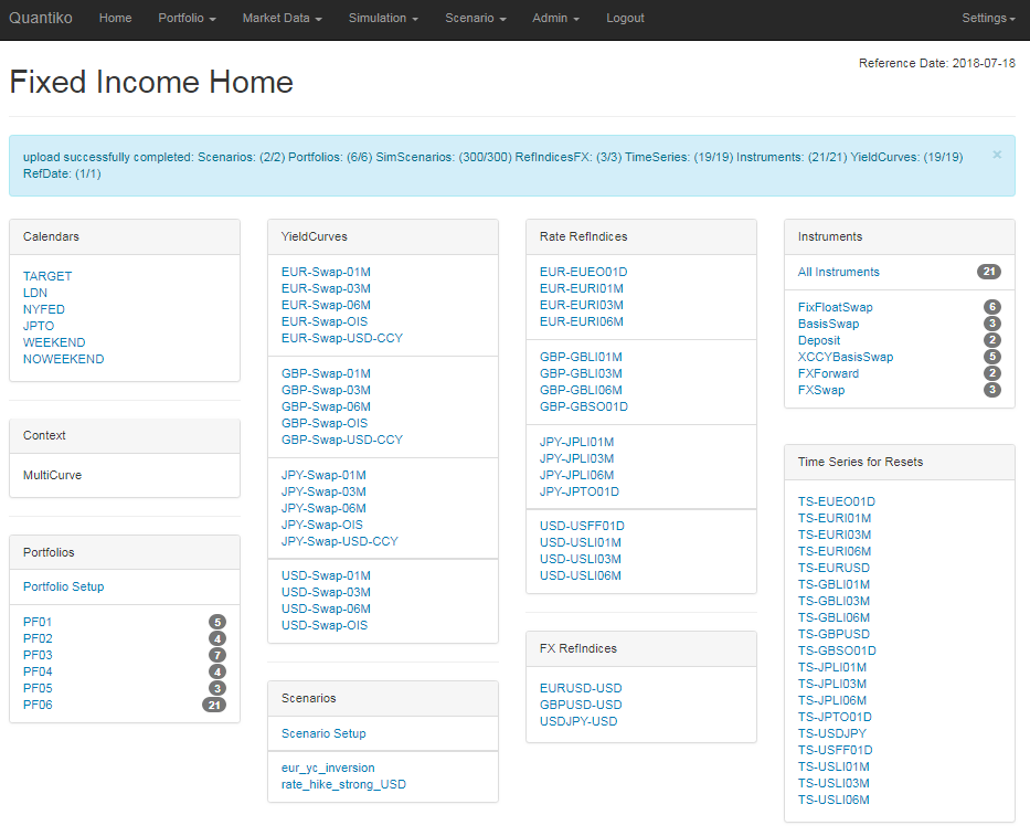
After login you arrive at the Home Screen with tiles containing links to calendars, market data objects for several currencies, instruments, portfolios and scenarios. At the top of the screen (as on any other screen) you see the black Navigation Bar. You will always get back to the Home Screen following the Home link in the Navigation Bar. In the upper right corner you find the Reference Date which is the date relative to which all calculations are carried out. Dates after that date are considered the future (with forward rates etc. estimated from market data objects), dates before that date are considered the past with fixing/reset values assumed to be known and available in TimeSeries objects. The other menu items on the Navigation Bar are:
Portfolio
Here you can create new portfolios and find shortcuts for the portfolios already defined.
Market Data
All yield curves and forward rate term structures are displayed, arranged by either currency or tenor.
Simulation
You can find all scenarios to be used in a simulation set by following Simulation → Simulation Scenarios. The simulation scenarios are used to estimate the loss distribution of a portfolio or an instrument. Additional parameters like quantiles or risk factors to be excluded from the simulation can be specified in Simulation → Quantile Set Parameters. Please be aware that simulation scenarios can only be uploaded from file.
Scenarios
Here you can define new market data (stress) scenarios and find shortcuts to the existing ones.
Admin
Here you can change your password, download files and upload data from files in JSON format.
Logout
Your current session ends and you are redirected. Please keep in mind that each user can only be logged in once at a time. If you attempt to login with your user, while being already logged in, the previous session will be terminated. Furthermore, after one hour of inactivity the current session will be terminated.
Setting
Here you can save your current session or load a previous session. There is one slot for a saved session available. Saving your session can be useful if you want to discuss an issue with an Admin User. Subject to your consent Admin Users are able to load your saved session and then see exactly what you are seeing. If you want to delete your current session, choose Settings → Flush Session. With Settings → Change Settings you can set the Reference Date without changing the market data set-up.
When you login for the first time, the Reference Date is set to the current date, all yield curves are flat at 0%, and all exchange rates are assumed to be 1. Since this initial set-up is slightly unrealistic and boring, we will show in the next section how you can easily upload a set of example market data to the service.
Getting Started: Create and Upload Data
Microsoft, Windows, Excel, and Visual Basic are trademarks or registered trademarks of Microsoft Corporation.
We provide an Excel spreadsheet with Visual Basic macros where you can enter market data (like yield curves and exchange rates) and instruments/trades, assign those trades to portfolios, and define market data scenarios. This tool then creates a file from the data in JSON format which you can upload to the service. A detailed description can be found here. Although you might also enter data in the service directly using web forms, the upload tool is more conventient for larger amounts of data or when the data is available in Excel anyway. The file to be uploaded can of course also be generated by other means than the upload tool, for instance by some piece of software which accesses a database directly and converts the retrieved data into the appropriate JSON format.
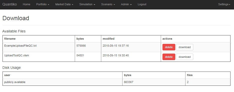
Step 1: Download the upload tool
Navigate to Admin → File Download and click on the download button for UploadToolQC.xlsm. Open the file and allow for macros. In case you do not have Excel available or do not want to activate macros you can download the example file ExampleUploadFileQC.txt instead and continue with Step 3.
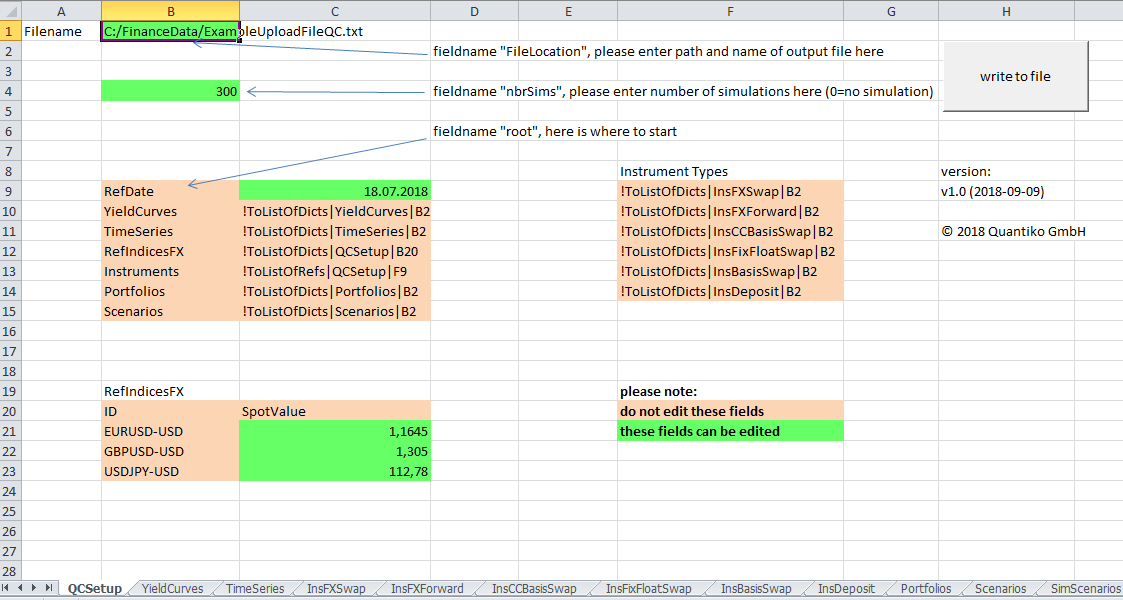
Step 2: Enter data in Excel and generate upload file
On tab QCSetup enter a valid path and filename in cell B1. The file to be uploaded will be stored at that location.
You can enter dates and numbers in the spreadsheet as usual in your locale. The upload tool will take care of this and converts into
ISO date format and numbers with decimal points. When you are done with editing or adding data
you might press the write to file
button. The file is now ready for upload at the specified location.
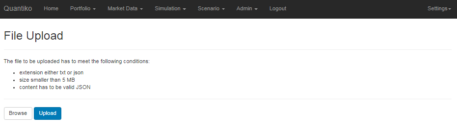
Step 3: Upload the file to the service
Go to Admin → File Upload, click on the Browse button, and navigate to the file to be uploaded. Press the Upload button. When the upload is completed you will be directed to the Home Screen with a message whether the upload has been successful or not.
Since the user-defined instrument identifier (alias
) has to be unique the service will complain when you try to upload instruments
with an existing alias once again.
In this case, make sure that you delete the current session by Settings → Flush Session first before you upload new data.
If you have not changed the data in the upload tool, the reference date will be set to 2018-07-18, and 21 instruments, 6 portfolios, 2 stress scenarios, and 300 simplistic simulation scenarios for EUR and USD yield curves and exchange rates have been generated for illustrative purposes. We are now ready to take a closer look at the market data objects and instruments in the next sections.
Market Data Objects
You can navigate to the market data objects below by following the links in the tiles on the Home Screen. Plots in the screens are mostly interactive, i.e. you can zoom in and out and drag the area shown. Hoovering with the mouse over a data point will show its coordinates.
Calendars
The calendar screen displays the business days for a given year in black and the non-business days in red. Default is the year of the Reference Date, but any year in a certain range can be chosen from the dropdown list at the top left corner.
Yield Curves
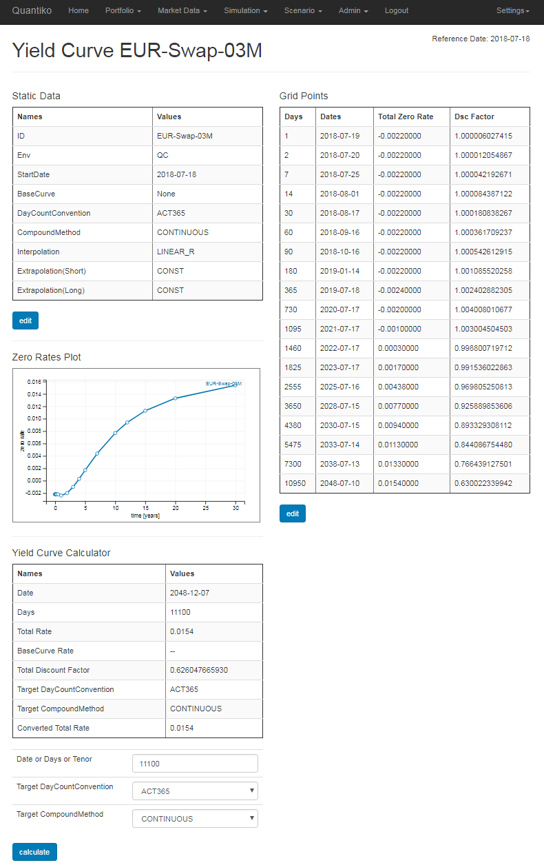
There is a set of built-in yield curves, basically Overnight-Index Swap (OIS) curves representing the risk-free rates and 1m, 3m, 6m tenor (zero) curves for the available currencies plus some cross currency curves for cashflows collateralized in USD. Currently, the yield curves are all base curves, spread curves are not supported yet.
Each yield curve consists of zero rates defined on given grid points together with an interpolation method which handles the calculation of zero rates between the grid points and extrapolation methods for going beyond the first and last grid point. In the Yield Curve Screen the grid points with corresponding zero rates and discount factors are shown in section Grid Points on the right hand side. Days are calendar days relative to the Reference Date and zero rates are understood to be in the day count and compounding conventions stated in section Static Data on the left. You can change day count and compounding conventions as well as the interpolation method when you click on the edit button in section Static Data. Please note that a change of day count or compounding convention will not affect the discount factors themselves, only the zero rates representing them.
Currently, linear and cubic spline interpolation is implemented — both on the zero rates themselves (..._R) and on the product of zero rate and time (..._RT).
You can add, modify or remove (by deleting the entry in column days) grid points with the edit button in section Grid Points. Displayed and entered rates are fractions of one, i.e. -0.01 corresponds to a zero rate of -1%.
In the lower section of the Yield Curve Screen you can find a calculator which displays the interpolated rate and discount factor for an arbitrary date. You can enter either a date, a tenor or the number of calendar days relative to Reference Date and choose a target day count and compounding convention. After clicking on the calculate button the zero rate in day count and compounding convention as defined in section Static Data and the discount factor are displayed under Total Rate and Total Discount Factor, respectively. In addition a converted zero rate into the target day count and compounding convention is shown under Converted Total Rate.
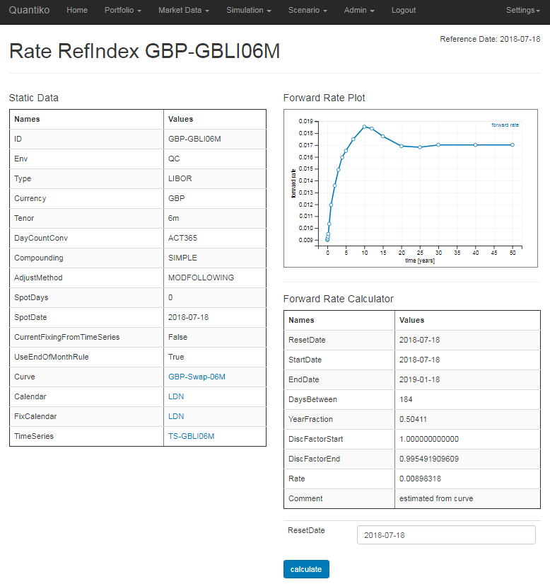
Rate Reference Indices
These market data objects are for estimating forward rates for a given tenor. The tenor and market conventions for quoting the forward rate are shown on the left hand side in section Static Data. The yield curve used for estimating the forward rate is displayed under Curve. For fixings/resets that are in the past relative to Reference Date a time series with historical values is needed — the connected time series is shown under TimeSeries. The field CurrentFixingFromTimeSeries determines whether a fixing/reset at Reference Date is taken from the time series or estimated from the yield curve.
There is also a forward rate calculator for a given reset/fixing date on the right hand side of the screen. Simply enter the reset/fixing date and click the calculate button, the calculated rate is displayed under Rate together with a comment whether the value is estimated from the yield curve or obtained from the connected time series.
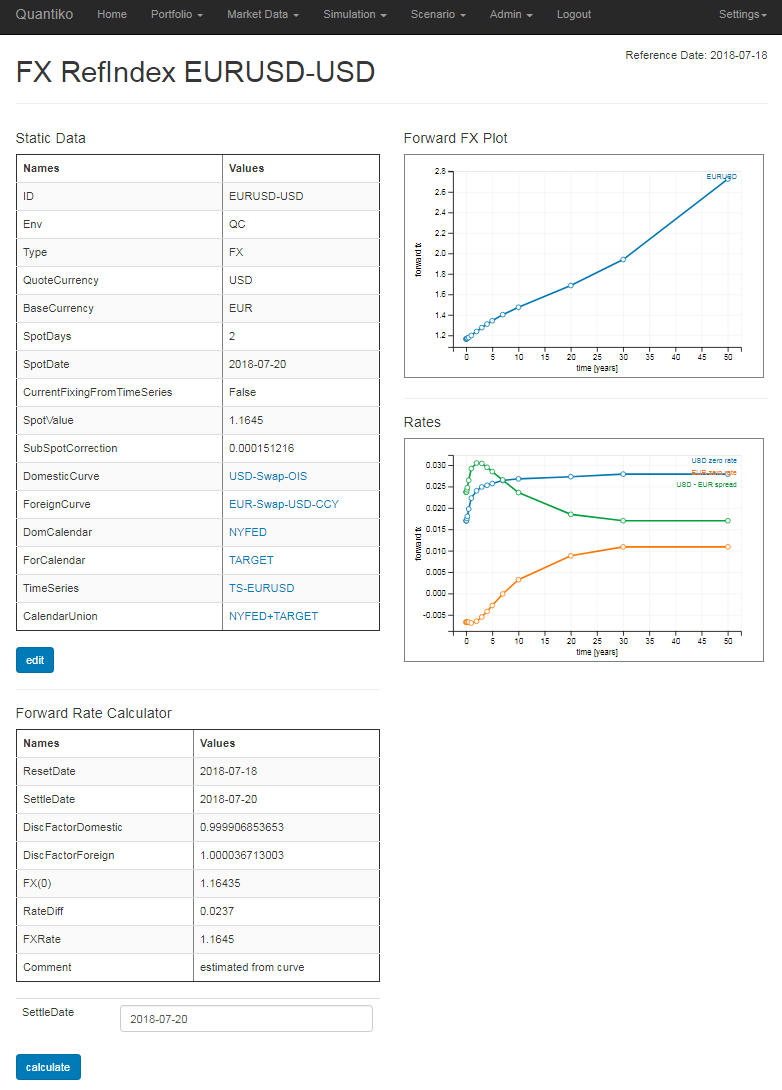
FX Reference Indices
FX Reference Indices estimate forward exchange rates of currency pairs. In contrast to Rate Reference Indices there is no tenor and two yield curves are necessary for estimating the forward exchange rate — following no-arbitrage arguments one for the quote (domestic) currency and one for the base (foreign) currency. The SpotValue shown in the Static Data section on the left is the current exchange rate observed on Reference Date for a spot transaction settling on SpotDate i.e. in SpotDays business days. By subtracting the SubSpotCorrection from the SpotValue the exchange rate of a (hypothetical) instantaneous transaction settling today is obtained. You can change the Spot Value with the edit button. For handling resets/fixings for dates in the past relative to Reference Date we also need a connected time series (TimeSeries). The time series value for a certain date might differ from the SpotValue used for that Reference Date.
There is also a forward rate calculator available on the left hand side which calculates the estimated forward exchange rate on any settlement date given. For instance if you enter the SpotDate here as settlement date, the forward exchange rate shown under FX Rate will by definition be identical to the SpotValue in section Static Data. FX(0) denotes the exchange rate of the instantaneous transaction settling at Reference Date.
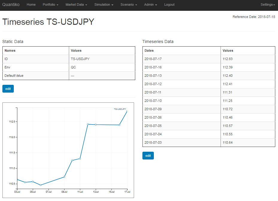
Time Series
For the valuation for financial instruments we might need historical fixing/reset values. There are Time Series Objects available for all Rate Reference Indices and FX Reference Indices. The actual historical values can be found on the right hand side of the Time Series Screen. You can add, modify or delete values by clicking on the edit button in the section Time Series Data.
On the left hand side the static data are shown. For each Time Series a default value can be set: whenever a historical fixing/reset value is needed the default value is used overriding the values in the section Time Series Data. The default value can be entered by clicking on the edit button in the section Static Data. The diagram will show a flat line with the default value in this case. When you want to use the time series on the right hand side again, simply remove the default value. Please keep in mind that most of the Time Series have a default value set in the example file obtained from the upload tool.
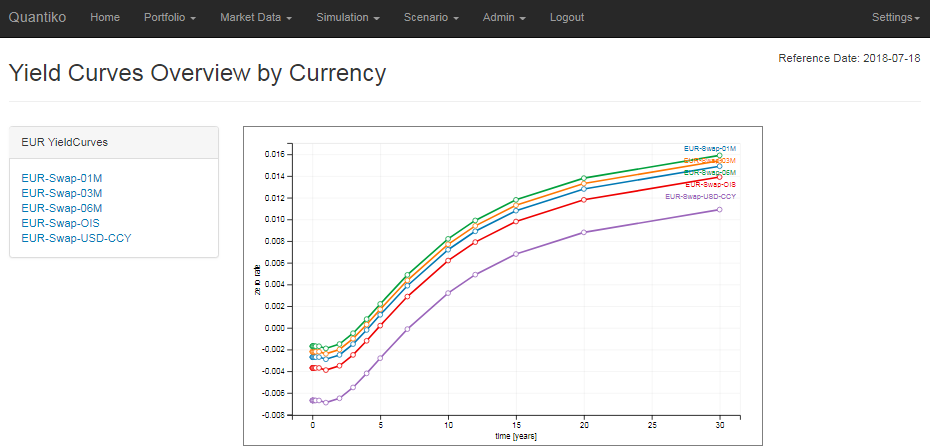
Term-Structure Plots for Currencies and Tenors
For assessing spreads between different tenors or interest rate levels between currencies it can be useful to have the term-structures of all yield curves of one currency or one tenor displayed in a single diagram. You can easily produce this type of analysis by following Market Data → Yield Curves per Ccy (Tenor) in the Navigation Bar. The same kind of plots but with forward rates instead of spot rates are available with Market Data → Rate Indices per Ccy (Tenor).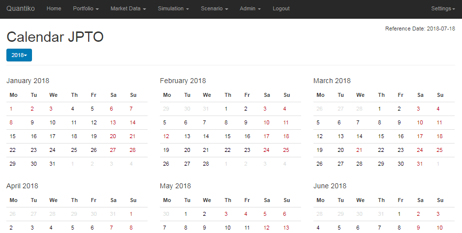
Instruments
In contrast to exchange traded securities where several trades can refer to one single instrument (for instance a bond) we consider here OTC derivatives where the trade specifics are individually negotiated between two counterparties and each trade refers to one instrument and one instrument only. For pure interest rate instruments (like an interest rate swap exchanging fix versus float coupon payments in the same currency) the trade currency is the currency of the rate reference index the instrument is referring to. For instruments involving a currency pair as underlying (like cross currency swap, FX swaps and FX forwards) the trade currency is assumed to be USD for the time being. We furthermore assume that the instruments/trades are fully collateralized with the trade currency being also the collateral currency.
At the moment the service supports the following instrument types:
- Single-Currency Interest Rate Swaps fix versus float
- Single-Currency Basis Swaps in Euro, US, and standard convention
- Fixed coupon interest rate payments
- Cross-Currency Basis Swaps in Reset Nominal (
Mark-To-Market
) and Constant Nominal convention - FX Forwards and FX Swaps
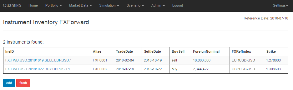
Instrument Inventory Screen
For each instrument type there is an inventory screen which lists all the existing instruments of that type — simply click on the link for that instrument type in the tile on the Home Screen. There is also a link for a screen with a list of all instruments. This screen contains a flush button which is conventient if you want to delete all instruments in one go.
In addition to the file upload you can also enter new instruments by clicking on the add button in each inventory screen. A description of the fields to be entered for each instrument type can be found here. A click on a link in the InsID column will direct you to the Instrument Screen with details and calculated values for that particular instrument.
The identifier or InsID of an instrument is automatically generated by the system using some of the instrument's data. You might however set a user-defined label in the Alias field, for instance some external reference number. Please note that this label has to be unique over all instruments.
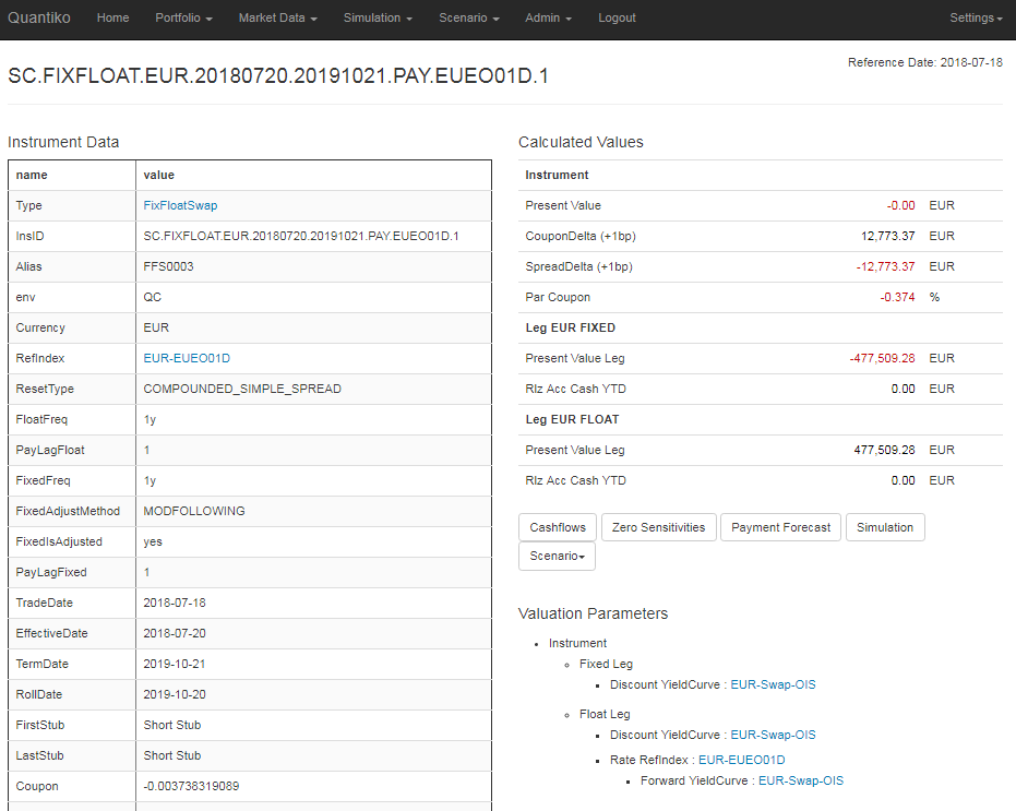
Instrument Screen
This screen consists of the instrument data on the left hand side and calculated values and mapped market data objects (section Valuation Parameters) on the right. You can modify instrument data or delete the instrument with the two buttons in section Instrument Data.
The items in the Calculated Values section depend on the instrument type. Usually, there is a present value in the trade currency of the instrument, some par rate or par spread which makes a similar instrument's present value zero, and a present value for each leg of the instrument. There are usually also some sensitivities shown: by how much does the present value change, when the FX rate (FXDelta), coupon (CouponDelta), spread (SpreadDelta) etc. changes by a certain amount.
The section Valuation Parameters shows all mapped market data objects necessary for the valuation of that instrument, like yield curves for discounting cashflows or yield curves for estimating forward (exchange) rates.
You can display the cashflows of the instrument by clicking on the Show Cashflows button. The button Show Zero Sensitivities will direct you to a screen which shows sensitivities with respect to yield curves shifts. The button Show Payment Forecast leads to a screen which shows the upcoming cash flows of the instrument. After clicking on the Simulation button the instrument is evaluated under all simulation scenarios defined. The same holds for the Scenario button where you can choose the scenario to be applied from a drop down list in the button.
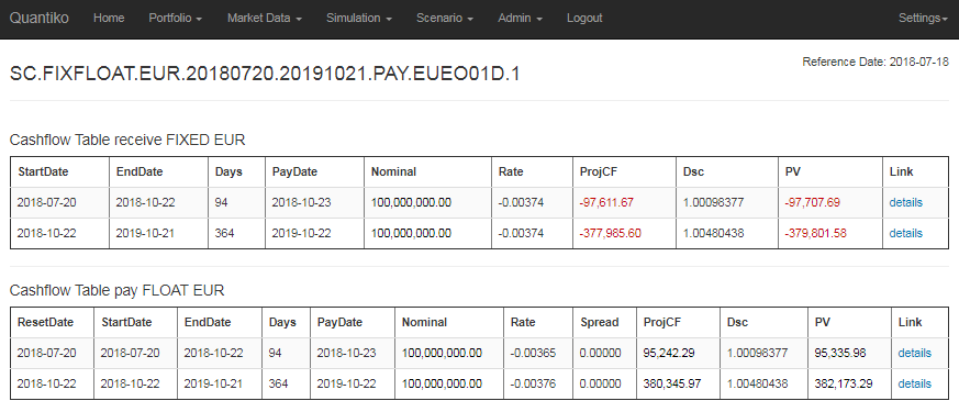
Cashflow and Cashflow Details Screens
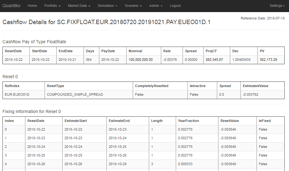
The cashflow screen displays cashflow tables for each leg of the instrument. The columns vary for different instrument types but usually you will find start and end date of the accrual period, pay date when the cashflow is due and one or more reset dates if the leg depends on reference indices. There is a column for the projected cashflow amount and its present value on Reference Date. The link in column Link will direct you to the cashflow details screen which provides additional information on that particular cashflow — for instance details on the multiple resets for a float rate cashflow in an Overnight Index Swap.
Zero Rate Sensitivities Screen
This screen shows the interest rate sensitivities of an instrument for all yield curves which are
necessary for valuation. The tables show bucket sensitivities: each grid point in a yield curve is shifted
separately by +1 basis point (bp) and the change in present value is observed. The upper part is on instrument
level (with the present value change understood to be in trade currency), the lower part is on leg
level (with the present value change understood to be in leg currency). Under each table the sum of
all buckets is displayed (sum
) and the change in present value when the curve as a whole is
uniformly shifted by +1 bp (shift
).
Payment Forecast Screen
The upcoming cashflows of an instrument over the next year are shown in this screen. Cashflows
are classified according to currency, realization (known
or estimated
for resets not yet fixed) and
type (principal
or interest
).
Portfolios
Instruments with an Alias label can be assigned to portfolios. An instrument might belong to several portfolios. You may define up to 10 portfolios. Each portfolio has a portfolio currency in order to aggregate quantities over instruments with different trade currencies.
Portfolio Setup
Following the Portfolio Setup link in the Home Screen or Portfolio → Portfolio Setup in the Navigation Bar will direct you to the place where you can manage your portfolios. You might add a new one and modify or delete an existing one by clicking the corresponding buttons. Deleting a portfolio will not affect the instruments that used to be assigned to that portfolio. To copy a portfolio with all its content, simply click on modify for the portfolio to be copied and enter a new name. Please note that you cannot add or modify a portfolio with a name which already exists.
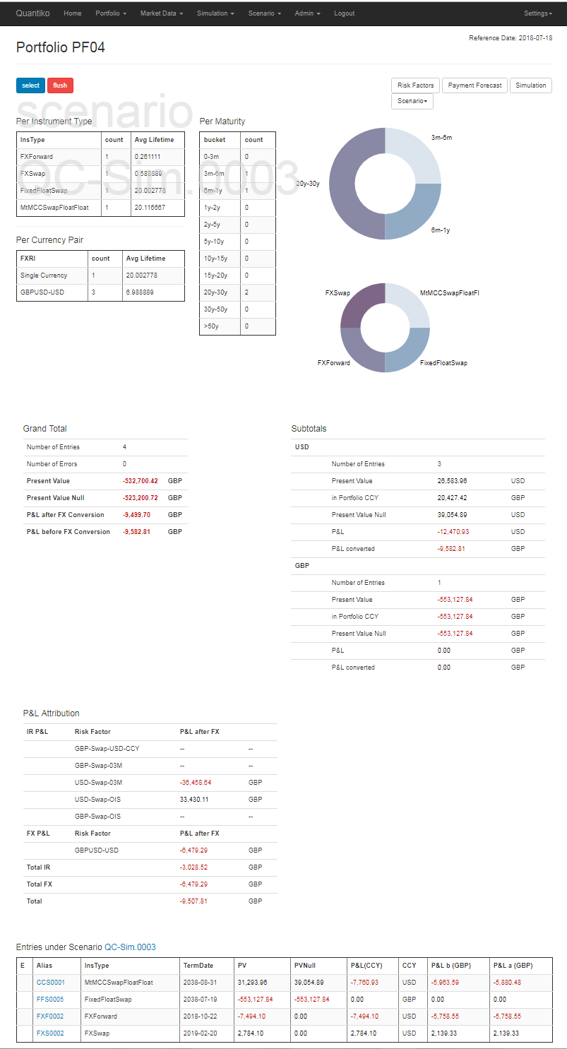
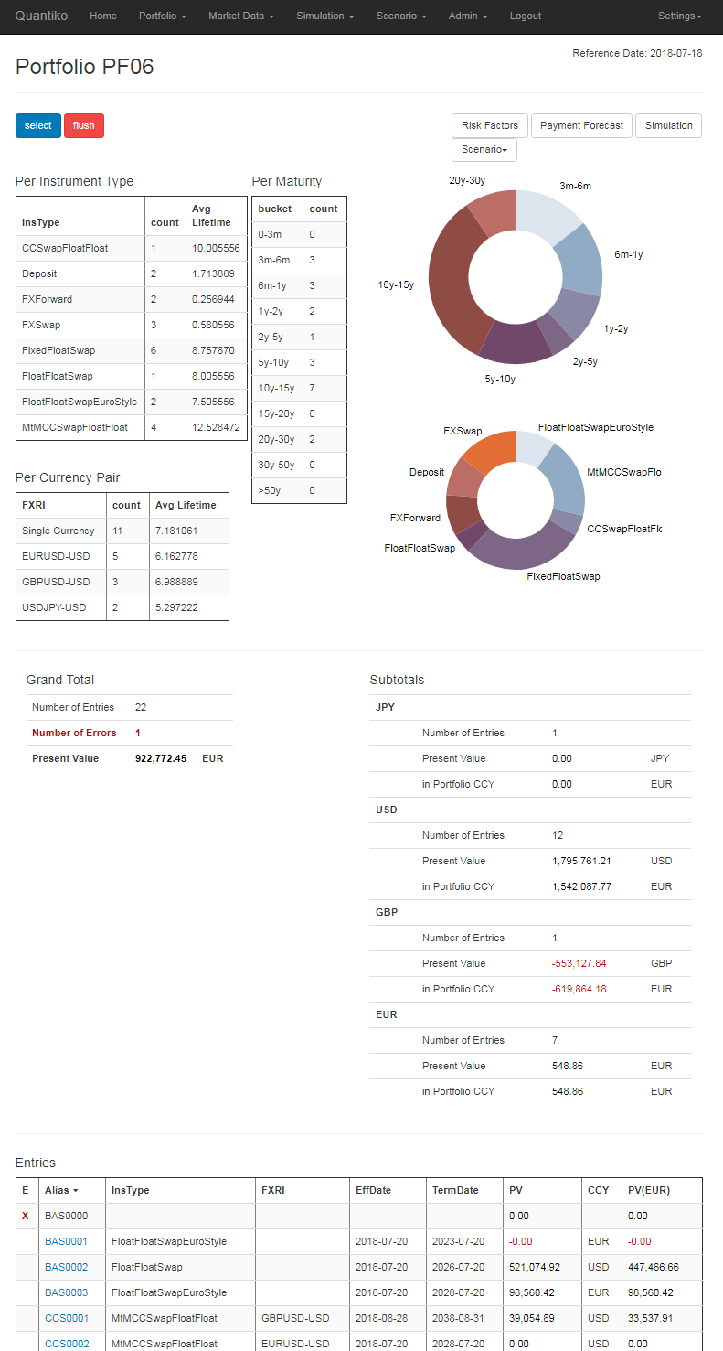
Portfolio Display
You arrive at the Portfolio Display screen by clicking on a link with the portfolio's name. In the upper part of the screen you find a breakdown of the portfolio into the categories Time to Maturity, Instrument Type and Currency Pairs. In the section Entries you see all the instruments assigned to that portfolio. The section Subtotals shows the aggregated present values for all trade currencies involved, while the section Grand Total converts these figures into the portfolio currency.
The button select at the top left will direct you to the Portfolio Definition screen where you can select the instruments in the portfolio. The flush button removes all instruments from the portfolio (without deleting the instruments themselves). The buttons at the top right will lead you to various analyses applied to the portfolio which are described below.
When for instance the alias of an instrument has changed, the instrument is deleted, or there are
market data (like fixings/reset values) missing, an error sign appears in the column E
of the table in section Entries.
By hoovering over the error sign the reason for the error is shown. The aggregated portfolio figures are nevertheless
calculated in this case, ignoring the instruments with errors.
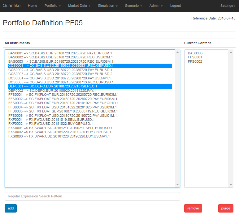
Portfolio Definition Screen
In this screen the portfolio content can be selected. In the left field of the screen you see all instruments that can be added to the portfolio (all instruments with an Alias label). In the right field the current content of the portfolio is shown. You can add instruments to the portfolio by highlighting them (keep the Ctrl key pressed in order to highlight more than one) in the left field and clicking on add. Instruments can be removed by highlighting them in the right field and clicking on remove. When you press the purge button, all instruments with errors are removed from the portfolio.
If you want to add instruments with a certain pattern in the Alias and/or Instrument Identifier you can enter a Regular Expression search pattern in the lower field and press the add button.
- To add all instruments containing pattern in Alias or Instrument Identifier enter .*pattern
- To add all instruments containing pattern in Alias alone enter [^>]*pattern
- To add all instruments containing pattern in Instrument Identifier alone enter .*>.*pattern
Portfolio Risk Factors
You arrive at this screen when you click on the Risk Factors
button in the Portfolio Display screen. All
relevant risk factors (yield curves and FX rates) of the portfolio are determined and the change in
present value in trade currency is calculated for each instrument (lower section Entries). For yield
curves the zero rates are uniformly shifted up by one basis point. FX rates are shifted up by 1%. The
aggregated value for each risk factor is shown in the upper section Totals.
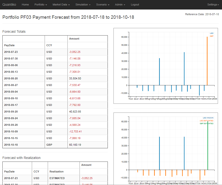
Portfolio Payment Forecast
You arrive at this screen when you click on the Payment Forecast
button in the Portfolio Display
screen. This screen offers a consolidated view on the upcoming cashflows over the next three month of
all instruments in the portfolio. Cashflows in each currency are classified into principal and
interest cashflows and whether the realization of the cashflow amount is known or
estimated. On the left side there are three tables with the cashflows aggregated according to
currency alone, currency and realization type, and currency, realization type and principal/interest.
The table at the bottom shows links to the instruments contributing to the cashflow of a particular
date. The pictures on the right which can be zoomed in x-direction visualize the information from the tables.
Scenarios
A scenario is a collection of shifts defined for some risk factors, that is yield curves and/or exchange rates.
You can apply a scenario to a portfolio or
a single instrument and find out how the shifted market data affects the present value and other calculated values. We define the
scenario P&L as the difference between the present value under the scenario and the present value in the unshifted case (null scenario
).
Often you assume for a scenario some extreme market moves which were observed in the past once or some hypothetical ones which you might fear to happen. The scenario P&L might then be used to quantify event risk (and for instance to limit trading activity) — although the likelihood of these rare events happening is hard to estimate. We refer to these kind of scenarios as What-If or Stress Scenarios.
If you apply a statistical ensemble of numerous scenarios to the portfolio or the instrument you will get a vector of scenario P&Ls which the associated market risk can be estimated from. A popular risk measure is the Value at Risk (VaR) which you obtain when you calculate the quantile for a given confidence level from the vector of scenario P&Ls. Usually the scenarios are constructed by applying the market moves over a given time horizont which were observed in the past to the current market environment (Historical Simulation) or by generating hypothetical market moves in a Monte Carlo engine with given probability distributions and dependencies. We refer to these kind of scenarios as Simulation Scenarios.
Since the service comes without an engine for Simulation Scenario generation you have to create them elsewhere and upload them to the service afterwards (the sheer amount of data makes the entry in web forms not feasible in our opinion). As an example how this could be done the upload tool creates simplistic Simulation Scenarios using a Monte Carlo engine.
The shifts to be applied to zero rates or exchange rates can be defined in three flavours (SpreadType
):
- Absolute Spread: the shift is interpreted as a spread to be added to the zero rate or the exchange rate of the null scenario. Example: an absolute spread of 0.001 on a zero rate of 2% means an upshift of 10 basis points, i.e. the zero rate increases to 2.1%.
- Relative Spread: the shift is interpreted as factor which the zero rate or the exchange rate of the null scenario is multipied with. Example: a relative spread of 0.9 on a zero rate of 2% means the zero rate decreases by 10% to 1.8%.
- Overwrite: the zero rate or the exchange rate of the null scenario is replaced by the shift. Example: an overwrite spread of 0.03 on a zero rate of 2% means the zero rate is now at 3%.
Since it is inconvenient to enter spreads for all grid points of a yield curve we apply linear or cubic spline interpolation between the specified spreads. The interpolated spreads are then applied to the intermediate grid points of the curve. Please note that the interpolation of zero rates between grid points is still determined by the interpolation type of the yield curve.
Scenario Setup
Following the Scenario Setup link in the Home Screen or Scenario → Scenario Setup in the Navigation Bar will direct you to the place where you can manage your stress scenarios. You might add a new one and modify or delete an existing one by clicking the corresponding buttons. To copy a scenario with all its market data shifts, simply click on modify for the scenario to be copied and enter a new name. Please note that you cannot add or modify a scenario with a name which already exists.
List of Simulation Scenarios
Following Simulation → Simulation Scenarios in the Navigation Bar you will see a table with all Simulation Scenarios defined on the left hand side of the screen. The link for each scenario will direct you to the Scenario Display Screen which shows all the risk factors and the applied shifts for that scenario. The table also displays the external label for each scenario, and the number of yield curves and exchange rates defined. The right hand side of the screen lists all risk factors involved and whether those risk factors are active or manually excluded from the Simulation Scenarios.
Simulation Scenarios are combined into so-called Quantile Sets. For each Quantile Set you can define a set of parameters for confidence levels, quantile calculation methods and risk factors to be excluded from the Simulation Scenarios. Those parameters can be managed by following Simulation → Quantile Set Parameters in the Navigation Bar.
Scenario Display Screen
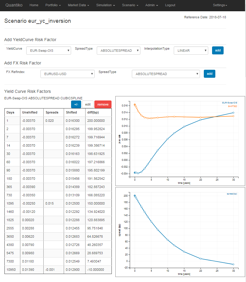
Both for Stress Scenarios and Simulation Scenarios you arrive at the Scenario Display screen by clicking on a link with the scenario's name. At the top of the screen you can add new yield curves or exchange rates to the scenario. In the lower part all yield curves and exchange rates which are part of the scenario are displayed. The plots show the yield curves shifted under the scenario and in the null scenario and the difference in basis points. By clicking on the +/- button you can unhide/hide a table showing the grid points of the yield curve with the unshifted zero rates, the specified shifts and the resulting shifted zero rates. With the edit button you can add, modify and delete the specified shifts. You can remove the yield curve or exchange rate from the scenario with the remove button.
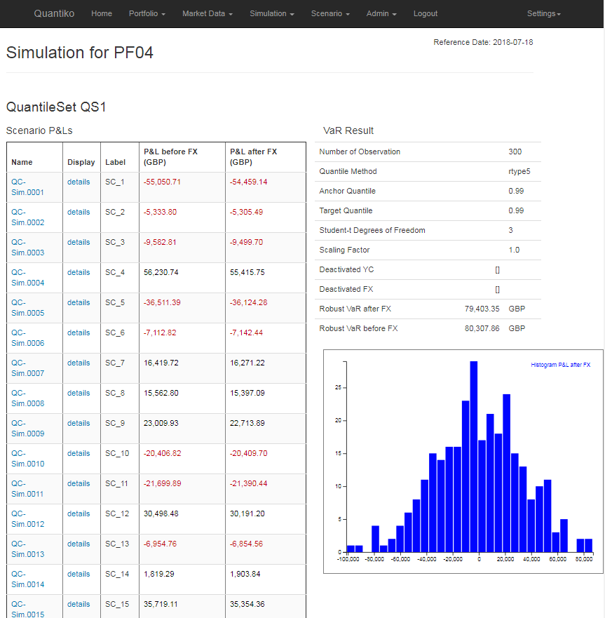
Portfolio Simulation
When you click on the Simulation button in the Portfolio Display screen the portfolio is evaluated under all Simulation Scenarios.
Depending on the number of instruments in the portfolio this might take a moment. On the left hand side of the Portfolio Simulation screen
you see a table with the scenario P&Ls under each Simulation Scenario in portfolio currency. The detail
links in the Display column will
direct you to a screen (similar to the Portfolio Display screen) with a detailed P&L attribution under that scenario. On the right hand side
you find the quantile set parameters used for the Value at Risk calculation and a histogram of the scenario P&Ls of the portfolio.
There are two ways to calculate the scenario P&L in portfolio currency for instruments with a trade currency different from the portfolio currency:
- You might first calculate the scenario P&L in trade currency and then convert this amount into portfolio currency with the scenario exchange rate. We will refer to this procedure as P&L before FX.
- You might convert the scenario present value in trade currency into portfolio currency with the scenario exchange rate first to find the scenario present value in portfolio currency. Then you convert the present value of the null scenario into portfolio currency with the exchange rate in the null scenario. Finally you calculate the difference of the two present values in portfolio currency. We will refer to this procedure as P&L after FX.
off-parthe instrument is in the null scenario. For an instrument at
parin the null scenario both scenario P&Ls will be the same. If trade currency is equal to portfolio currency the two P&L numbers will always be the same.
Portfolio P&L Attribution
You will reach this screen by either clicking on the details
link in the Portfolio Simulation screen or by choosing a Stress Scenario
on the scenario button in the Portfolio Display screen. The portfolio is evaluated under the Simulation or Stress Scenario, respectively,
and the scenario P&L is then attributed to separate shifts for all risk factors involved.
The P&L before FX and P&L after FX values are shown in Grand Total section on the left hand side of the screen. The P&L before FX values broken down to trade currencies are displayed in section Subtotals on the right hand side. In section P&L Attribution each yield curve and exchange rate the portfolio is depending on is shifted separately and the P&L after FX value is displayed. Please note that for a necessary conversion from trade currency into portfolio currency the exchange rate for the null scenario is used here. Hence the sum of all contributions in line Total might differ from the P&L after FX value in section Grand Total due to the currency conversion and also due to cross gamma effects.
The table at the bottom of the screen shows the P&Ls for each instrument in the portfolio. Clicking on the instrument alias will direct you to the Instrument P&L Attribution screen.
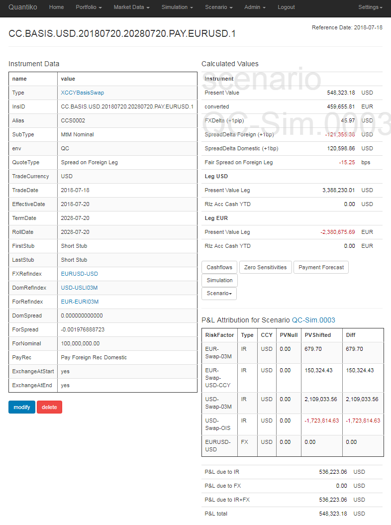
Instrument P&L Attribution
Here a single instrument is evaluated under a Simulation or Stress Scenario and the P&L in trade currency is then attributed to separate shifts for all risk factors involved. If you follow the links for Cashflow Table and Cashflow Forecast from this screen the resulting tables are calculated under the corresponding scenario as recognisable from the watermark with the scenario's name on the screen.